Examples

See also

Quickstart for a quick introduction. MCMC Parameter Fitting for parameter fitting. Parameter Reference for parameter details.

Basic Usage

Setting up a simple afterglow model

import matplotlib.pyplot as plt
import numpy as np
from VegasAfterglow import ISM, TophatJet, Observer, Radiation, Model

# Define the circumburst environment (constant density ISM)
medium = ISM(n_ism=1)

# Configure the jet structure (top-hat with opening angle, energy, and Lorentz factor)
jet = TophatJet(theta_c=0.1, E_iso=1e52, Gamma0=300)

# Set observer parameters (distance, redshift, viewing angle)
obs = Observer(lumi_dist=1e26, z=0.1, theta_obs=0)

# Define radiation microphysics parameters
rad = Radiation(eps_e=1e-1, eps_B=1e-3, p=2.3, xi_e=1)

# Combine all components into a complete afterglow model
model = Model(jet=jet, medium=medium, observer=obs, fwd_rad=rad, resolutions=(0.15,0.5,10))

# Define time range for light curve calculation
times = np.logspace(2, 8, 200)

# Define observing frequencies (radio, optical, X-ray bands in Hz)
bands = np.array([1e9, 1e14, 1e17])

# Calculate the afterglow emission at each time and frequency
# NOTE that the times array needs to be in ascending order
results = model.flux_density_grid(times, bands)

# Visualize the multi-wavelength light curves
plt.figure(figsize=(4.8, 3.6),dpi=200)

# Plot each frequency band
for i, nu in enumerate(bands):
    exp = int(np.floor(np.log10(nu)))
    base = nu / 10**exp
    plt.loglog(times, results.total[i,:], label=fr'${base:.1f} \times 10^{{{exp}}}$ Hz')

plt.xlabel('Time (s)')
plt.ylabel('Flux Density (erg/cm²/s/Hz)')
plt.legend()

# Define broad frequency range (10⁵ to 10²² Hz)
frequencies = np.logspace(5, 22, 200)

# Select specific time epochs for spectral snapshots
epochs = np.array([1e2, 1e3, 1e4, 1e5 ,1e6, 1e7, 1e8])

# Calculate spectra at each epoch
results = model.flux_density_grid(epochs, frequencies)

# Plot broadband spectra at each epoch
plt.figure(figsize=(4.8, 3.6),dpi=200)
colors = plt.cm.viridis(np.linspace(0,1,len(epochs)))

for i, t in enumerate(epochs):
    exp = int(np.floor(np.log10(t)))
    base = t / 10**exp
    plt.loglog(frequencies, results.total[:,i], color=colors[i], label=fr'${base:.1f} \times 10^{{{exp}}}$ s')

# Add vertical lines marking the bands from the light curve plot
for i, band in enumerate(bands):
    exp = int(np.floor(np.log10(band)))
    base = band / 10**exp
    plt.axvline(band,ls='--',color='C'+str(i))

plt.xlabel('frequency (Hz)')
plt.ylabel('flux density (erg/cm²/s/Hz)')
plt.legend(ncol=2)
plt.title('Synchrotron Spectra')

Calculate flux on time-frequency pairs

Suppose you want to calculate the flux at specific time-frequency pairs (t_i, nu_i) instead of a grid (t_i, nu_j), you can use the following method:

# Define time range for light curve calculation
times = np.logspace(2, 8, 200)

# Define observing frequencies (must be the same length as times)
bands = np.logspace(9,17, 200)

results = model.flux_density(times, bands) #times array must be in ascending order

# the returned results is a FluxDict object with arrays of the same shape as the input times and bands.

Calculate flux with exposure time averaging

For observations with finite exposure times, you can calculate time-averaged flux by sampling multiple points within each exposure:

# Define observation times (start of exposure)
times = np.logspace(2, 8, 50)

# Define observing frequencies (must be the same length as times)
bands = np.logspace(9, 17, 50)

# Define exposure times for each observation (in seconds)
expo_time = np.ones_like(times) * 100  # 100-second exposures

# Calculate time-averaged flux with 20 sample points per exposure
results = model.flux_density_exposures(times, bands, expo_time, num_points=20)

# The returned results is a FluxDict object with arrays of the same shape as input times and bands
# Each flux value represents the average over the corresponding exposure time

Note

The function samples num_points evenly spaced within each exposure time and averages the computed flux. Higher num_points gives more accurate time averaging but increases computation time. The minimum value is 2.

Calculate bolometric flux (frequency-integrated)

For broadband flux measurements integrated over a frequency range (e.g., instrument bandpasses like Swift/BAT, Fermi/LAT):

# Define time range for broadband light curve calculation
times = np.logspace(2, 8, 100)

# Example 1: Swift/BAT bandpass (15-150 keV ≈ 3.6e18 - 3.6e19 Hz)
nu_min_bat = 3.6e18  # Lower frequency bound [Hz]
nu_max_bat = 3.6e19  # Upper frequency bound [Hz]
num_points = 20      # Number of frequency sampling points for integration

# Calculate frequency-integrated flux
flux_bat = model.flux(times, nu_min_bat, nu_max_bat, num_points)

# Example 2: Custom optical band (V-band: 5.1e14 ± 5e13 Hz)
nu_min_v = 4.6e14    # V-band lower edge [Hz]
nu_max_v = 5.6e14    # V-band upper edge [Hz]
flux_v = model.flux(times, nu_min_v, nu_max_v, num_points)

# Plot broadband light curves
plt.figure(figsize=(8, 6))
plt.loglog(times, flux_bat.total, label='Swift/BAT (15-150 keV)', linewidth=2)
plt.loglog(times, flux_v.total, label='V-band optical', linewidth=2)

plt.xlabel('Time [s]')
plt.ylabel('Integrated Flux [erg/cm²/s]')
plt.legend()
plt.title('Broadband Light Curves')

Note

When to use `flux` vs `flux_density_grid`:

• Use flux() for broadband flux measurements (instrument bandpasses, bolometric calculations)

• Use flux_density_grid() for monochromatic flux densities at specific frequencies

• The flux() method integrates over frequency, so units are [erg/cm²/s] instead of [erg/cm²/s/Hz]

• Higher num_points gives more accurate frequency integration but increases computation time

Tip

Frequency Integration Guidelines:

• Narrow bands (Δν/ν < 0.5): Use num_points = 5-10

• Wide bands (Δν/ν > 1): Use num_points = 20-50

• Very wide bands (multiple decades): Use num_points = 50+

• Monitor convergence by testing different num_points values

Ambient Media Models

Wind Medium

from VegasAfterglow import Wind

# Create a stellar wind medium
wind = Wind(A_star=0.1)  # A* parameter

#..other settings
model = Model(medium=wind, ...)

Stratified Medium

from VegasAfterglow import Wind

# Create a stratified stellar wind medium;
# smooth transited stratified medium. Inner region, n(r) = n0, middle region n(r) \propto 1/r^2, outer region n(r)=n_ism
# A = 0 (default): fallback to n = n_ism
# n0 = inf (default): wind bubble, from wind profile to ism profile
# A = 0 & n0 = inf: pure wind;
wind = Wind(A_star=0.1, n_ism = 1, n0 = 1e3)

#..other settings
model = Model(medium=wind, ...)

User-Defined Medium

from VegasAfterglow import Medium

mp = 1.67e-24 # proton mass in gram

# Define a custom density profile function
def density(phi, theta, r):# r in cm, phi and theta in radians [scalar]
    return mp # n_ism =  1 cm^-3
    #return whatever density profile (g*cm^-3) you want as a function of phi, theta, and r

# Create a user-defined medium
medium = Medium(rho=density)

#..other settings
model = Model(medium=medium, ...)

Jet Models

Gaussian Jet

from VegasAfterglow import GaussianJet

# Create a structured jet with Gaussian energy profile
jet = GaussianJet(
    theta_c=0.05,         # Core angular size (radians)
    E_iso=1e53,           # Isotropic-equivalent energy (ergs)
    Gamma0=300            # Initial Lorentz factor
)

#..other settings
model = Model(jet=jet, ...)

Power-Law Jet

from VegasAfterglow import PowerLawJet

# Create a power-law structured jet
jet = PowerLawJet(
    theta_c=0.05,         # Core angular size (radians)
    E_iso=1e53,           # Isotropic-equivalent energy (ergs)
    Gamma0=300,           # Initial Lorentz factor
    k_e=2.0,              # Power-law index for energy angular dependence
    k_g=2.0               # Power-law index for Lorentz factor angular dependence
)

#..other settings
model = Model(jet=jet, ...)

Two-Component Jet

from VegasAfterglow import TwoComponentJet

# Create a two-component jet
jet = TwoComponentJet(
    theta_c=0.05,        # Narrow component angular size (radians)
    E_iso=1e53,          # Isotropic-equivalent energy of the narrow component (ergs)
    Gamma0=300,          # Initial Lorentz factor of the narrow component
    theta_w=0.1,         # Wide component angular size (radians)
    E_iso_w=1e52,        # Isotropic-equivalent energy of the wide component (ergs)
    Gamma0_w=100         # Initial Lorentz factor of the wide component
)

#..other settings
model = Model(jet=jet, ...)

Step Power-Law Jet

from VegasAfterglow import StepPowerLawJet

# Create a step power-law structured jet (uniform core with sharp transition)
jet = StepPowerLawJet(
    theta_c=0.05,        # Core angular size (radians)
    E_iso=1e53,          # Isotropic-equivalent energy of the core component (ergs)
    Gamma0=300,          # Initial Lorentz factor of the core component
    E_iso_w=1e52,        # Isotropic-equivalent energy of the wide component (ergs)
    Gamma0_w=100,        # Initial Lorentz factor of the wide component
    k_e=2.0,             # Power-law index for energy angular dependence
    k_g=2.0              # Power-law index for Lorentz factor angular dependence
)

#..other settings
model = Model(jet=jet, ...)

Jet with Spreading

from VegasAfterglow import TophatJet

jet = TophatJet(
    theta_c=0.05,
    E_iso=1e53,
    Gamma0=300,
    spreading=True       # Enable spreading
)

#..other settings
model = Model(jet=jet, ...)

Note

The jet spreading (Lateral Expansion) is experimental and only works for the top-hat jet, Gaussian jet, and power-law jet with a jet core. The spreading prescription may not work for arbitrary user-defined jet structures.

Magnetar Spin-down

from VegasAfterglow import Magnetar

# Create a tophat jet with magnetar spin-down energy injection; Luminosity 1e46 erg/s, t_0 = 100 seconds, and q = 2
jet = TophatJet(theta_c=0.05, E_iso=1e53, Gamma0=300, magnetar=Magnetar(L0=1e46, t0=100, q=2))

Note

The magnetar spin-down injection is implemented in the default form L0*(1+t/t0)^(-q) for theta < theta_c. You can pass the magnetar argument to the power-law and Gaussian jet as well.

User-Defined Jet

You may also define your own jet structure by providing the energy and lorentz factor profile. Those two profiles are required to complete a jet structure. You may also provide the magnetization profile, enregy injection profile, and mass injection profile. Those profiles are optional and will be set to zero function if not provided.

from VegasAfterglow import Ejecta

# Define a custom energy profile function, required to complete the jet structure
def E_iso_profile(phi, theta):
    return 1e53  # E_iso = 1e53 erg isotropic fireball
    #return whatever energy profile you want as a function of phi and theta in unit of erg [not erg per solid angle]

# Define a custom lorentz factor profile function, required to complete the jet structure
def Gamma0_profile(phi, theta):
    return 300 # Gamma0 = 300
    #return whatever lorentz factor profile you want as a function of phi and theta

# Define a custom magnetization profile function, optional
def sigma0_profile(phi, theta):
    return 0.1 # sigma = 0.1
    #return whatever magnetization profile you want as a function of phi and theta

# Define a custom energy injection profile function, optional
def E_dot_profile(phi, theta, t):
    return 1e46 * (1 + t / 100)**(-2) # L = 1e46 erg/s, t0 = 100 seconds
    #return whatever energy injection  profile you want as a function of phi, theta, and time in unit of erg/s [not erg/s per solid angle]

# Define a custom mass injection profile function, optional
def M_dot_profile(phi, theta, t):
    #return whatever mass injection profile you want as a function of phi, theta, and time in unit of g/s [not g/s per solid angle]

# Create a user-defined jet
jet = Ejecta(E_iso=E_iso_profile, Gamma0=Gamma0_profile, sigma0=sigma0_profile, E_dot=E_dot_profile, M_dot=M_dot_profile)

#..other settings

#if your jet is not axisymmetric, set axisymmetric to False
model = Model(jet=jet, ..., axisymmetric=False, resolutions=(0.15, 0.5, 10))

# the user-defined jet structure could be spiky, the default resolution may not resolve the jet structure. if that is the case, you can try a finer resolution (phi_ppd, theta_ppd, t_ppd)
# where phi_ppd is the number of points per degree in the phi direction, theta_ppd is the number of points per degree in the theta direction, and t_ppd is the number of points per decade in the time direction    .

Note

Plain Python callbacks work well for single model evaluations (light curves, spectra). For multi-threaded MCMC fitting, use the @gil_free decorator to compile your profile functions to native code, eliminating GIL contention across threads. See the GIL-Free Native Callbacks section below and MCMC Parameter Fitting for details.

GIL-Free Native Callbacks (@gil_free)

When C++ evaluates a plain Python callback (e.g., a custom jet or medium profile), it must acquire the Global Interpreter Lock (GIL) for every call. During blast wave evolution this happens hundreds of times per model evaluation, which serializes the angular-profile loop across threads.

The @gil_free decorator compiles a Python function to native machine code via numba, so C++ calls it directly as a C function pointer — no GIL, no interpreter overhead:

pip install numba

Key differences from plain Python callbacks:

1. Decorate with @gil_free

2. Physical parameters come as extra function arguments (after the spatial coordinates) instead of being captured from the enclosing scope

3. Call the decorated function with keyword arguments to bind parameters — this returns a NativeFunc object that C++ can call at full speed

4. Only math module functions and simple arithmetic are allowed (no numpy arrays, no Python objects)

Working example — Gaussian jet + wind medium:

import math
import numpy as np
import matplotlib.pyplot as plt
from VegasAfterglow import Ejecta, Medium, Observer, Radiation, Model, gil_free

@gil_free
def gaussian_energy(phi, theta, E_iso, theta_c):
    return E_iso * math.exp(-0.5 * (theta / theta_c) ** 2)

@gil_free
def gaussian_gamma(phi, theta, Gamma0, theta_c):
    return 1.0 + (Gamma0 - 1.0) * math.exp(-0.5 * (theta / theta_c) ** 2)


@gil_free
def wind_density(phi, theta, r, A_star):
    mp = 1.67e-24
    return A_star * 5e11 * mp / (r * r)

# --- Build the model ---
# Calling the decorated function with keyword arguments binds those parameters
# and returns a NativeFunc. You can bind as many parameters as you need —
# they just need to appear after the spatial coordinates in the function signature.
# This is especially useful for MCMC, where you rebind parameters each step.

E_iso = 1e52      # these could come from MCMC sampler
Gamma0 = 300
theta_c = 0.1
A_star = 0.1

jet = Ejecta(
    E_iso=gaussian_energy(E_iso=E_iso, theta_c=theta_c),
    Gamma0=gaussian_gamma(Gamma0=Gamma0, theta_c=theta_c),
)

medium = Medium(rho=wind_density(A_star=A_star))
obs = Observer(lumi_dist=1e26, z=0.1, theta_obs=0.3)
rad = Radiation(eps_e=0.1, eps_B=1e-3, p=2.3)

model = Model(jet=jet, medium=medium, observer=obs, fwd_rad=rad)

times = np.logspace(2, 8, 100)
bands = np.array([1e9, 1e14, 1e17])
results = model.flux_density_grid(times, bands)

for i, nu in enumerate(bands):
    plt.loglog(times, results.total[i, :])
plt.xlabel('Time (s)')
plt.ylabel('Flux Density (erg/cm²/s/Hz)')
plt.show()

Tip

Functions decorated with @gil_free must only use the math module (not numpy) and simple arithmetic — no Python objects, arrays, or closures. If you need more complex logic, use the plain Python callback approach instead.

Note

Built-in jet types (TophatJet, GaussianJet, PowerLawJet, etc.) are already implemented in C++ and do not need this decorator. Use @gil_free only for custom profiles passed via Ejecta or Medium.

Radiation Processes

Reverse Shock Emission

from VegasAfterglow import Radiation

#set the jet duration to be 100 seconds, the default is 1 second. The jet duration affects the reverse shock thickness (thin shell or thick shell).
jet = TophatJet(theta_c=0.1, E_iso=1e52, Gamma0=300, duration = 100)

# Create a radiation model with both forward and reverse shock synchrotron radiation
fwd_rad = Radiation(eps_e=1e-1, eps_B=1e-3, p=2.3)
rvs_rad = Radiation(eps_e=1e-2, eps_B=1e-4, p=2.4)

#..other settings
model = Model(fwd_rad=fwd_rad, rvs_rad=rvs_rad, resolutions=(0.15, 0.5, 10),...)

times = np.logspace(2, 8, 200)

bands = np.array([1e9, 1e14, 1e17])

results = model.flux_density_grid(times, bands)

plt.figure(figsize=(4.8, 3.6),dpi=200)

# Plot each frequency band
for i, nu in enumerate(bands):
    exp = int(np.floor(np.log10(nu)))
    base = nu / 10**exp
    plt.loglog(times, results.fwd.sync[i,:], label=fr'${base:.1f} \times 10^{{{exp}}}$ Hz (fwd)')
    plt.loglog(times, results.rvs.sync[i,:], label=fr'${base:.1f} \times 10^{{{exp}}}$ Hz (rvs)')#reverse shock synchrotron

Note

You may increase the resolution of the grid to improve the accuracy of the reverse shock synchrotron radiation if you see spiky features.

Inverse Compton Cooling

from VegasAfterglow import Radiation

# Create a radiation model with SSC and IC cooling (without Klein-Nishina correction)
rad = Radiation(eps_e=1e-1, eps_B=1e-3, p=2.3, ssc=True, kn=False)

#..other settings
model = Model(fwd_rad=rad, ...)

Self-Synchrotron Compton Radiation

from VegasAfterglow import Radiation

# Create a radiation model with self-Compton radiation and Klein-Nishina corrections
rad = Radiation(eps_e=1e-1, eps_B=1e-3, p=2.3, ssc=True, kn=True)

#..other settings
model = Model(fwd_rad=rad, ...)

times = np.logspace(2, 8, 200)

bands = np.array([1e9, 1e14, 1e17])

results = model.flux_density_grid(times, bands)

plt.figure(figsize=(4.8, 3.6),dpi=200)

# Plot each frequency band
for i, nu in enumerate(bands):
    exp = int(np.floor(np.log10(nu)))
    base = nu / 10**exp
    plt.loglog(times, results.fwd.sync[i,:], label=fr'${base:.1f} \times 10^{{{exp}}}$ Hz (sync)')#synchrotron
    plt.loglog(times, results.fwd.ssc[i,:], label=fr'${base:.1f} \times 10^{{{exp}}}$ Hz (SSC)')#SSC

Note

When ssc=True, IC cooling of electrons is automatically included. The kn flag controls whether Klein-Nishina corrections are applied:

(ssc = True, kn = False): SSC emission with IC cooling using the Thomson cross-section.

(ssc = True, kn = True): SSC emission with IC cooling and Klein-Nishina corrections.

For details on the underlying radiation physics, see GRB Afterglow Physics.

Internal Quantities Evolution

This section demonstrates advanced access to internal simulation quantities. For basic model setup, see Quickstart.

VegasAfterglow provides comprehensive access to internal simulation quantities, allowing you to analyze the temporal evolution of physical parameters across different reference frames. This enables detailed investigation of shock dynamics, microphysical parameters, and relativistic effects throughout the afterglow evolution.

Model Setup for Internal Analysis

Similar to the light curve generation, let’s set up the physical components of our afterglow model with additional resolution parameters for detailed internal tracking:

import numpy as np
import matplotlib.pyplot as plt
from VegasAfterglow import ISM, TophatJet, Observer, Radiation, Model

medium = ISM(n_ism=1)
jet = TophatJet(theta_c=0.3, E_iso=1e52, Gamma0=100)
z = 0.1
obs = Observer(lumi_dist=1e26, z=z, theta_obs=0.)
rad = Radiation(eps_e=1e-1, eps_B=1e-3, p=2.3)

# Include resolution parameters for detailed internal tracking
model = Model(jet=jet, medium=medium, observer=obs, fwd_rad=rad, resolutions=(0.15,0.5,10))

Accessing Simulation Quantities

Now, let’s access the internal simulation quantities using the details method:

# Get the simulation details over a time range
details = model.details(t_min=1e0, t_max=1e8)

# Print the available attributes
print("Simulation details attributes:", dir(details))
print("Forward shock attributes:", dir(details.fwd))

You will get a SimulationDetails object with the following structure:

Main grid coordinates:

• details.phi: 1D numpy array of azimuthal angles in radians

• details.theta: 1D numpy array of polar angles in radians

• details.t_src: 3D numpy array of source frame times on coordinate (phi_i, theta_j, t_k) grid in seconds

Forward shock details (accessed via ``details.fwd``):

• details.fwd.t_comv: 3D numpy array of comoving times for the forward shock in seconds

• details.fwd.t_obs: 3D numpy array of observer times for the forward shock in seconds

• details.fwd.Gamma: 3D numpy array of downstream Lorentz factors for the forward shock

• details.fwd.Gamma_th: 3D numpy array of thermal Lorentz factors for the forward shock

• details.fwd.r: 3D numpy array of lab frame radii in centimeters

• details.fwd.B_comv: 3D numpy array of downstream comoving magnetic field strengths for the forward shock in Gauss

• details.fwd.theta: 3D numpy array of polar angles for the forward shock in radians

• details.fwd.N_p: 3D numpy array of downstream shocked proton number per solid angle for the forward shock

• details.fwd.N_e: 3D numpy array of downstream synchrotron electron number per solid angle for the forward shock

• details.fwd.gamma_a: 3D numpy array of comoving frame self-absorption Lorentz factors for the forward shock

• details.fwd.gamma_m: 3D numpy array of comoving frame injection Lorentz factors for the forward shock

• details.fwd.gamma_c: 3D numpy array of comoving frame cooling Lorentz factors for the forward shock

• details.fwd.gamma_M: 3D numpy array of comoving frame maximum Lorentz factors for the forward shock

• details.fwd.nu_a: 3D numpy array of comoving frame self-absorption frequencies for the forward shock in Hz

• details.fwd.nu_m: 3D numpy array of comoving frame injection frequencies for the forward shock in Hz

• details.fwd.nu_c: 3D numpy array of comoving frame cooling frequencies for the forward shock in Hz

• details.fwd.nu_M: 3D numpy array of comoving frame maximum frequencies for the forward shock in Hz

• details.fwd.I_nu_max: 3D numpy array of comoving frame synchrotron maximum specific intensities for the forward shock in erg/cm²/s/Hz

• details.fwd.Doppler: 3D numpy array of Doppler factors for the forward shock

• details.fwd.sync_spectrum: Per-cell callable synchrotron spectrum (see Per-Cell Spectrum Evaluation)

• details.fwd.ssc_spectrum: Per-cell callable SSC spectrum (None if ssc=False)

• details.fwd.Y_spectrum: Per-cell callable Compton-Y parameter

Reverse shock details (accessed via ``details.rvs``, if reverse shock is enabled):

• Similar attributes as forward shock but for the reverse shock component

Multi-Parameter Evolution Visualization

To analyze the temporal evolution of physical parameters across different reference frames, we can visualize how key quantities evolve in the source frame, comoving frame, and observer frame. This code creates a comprehensive multi-panel figure displaying the temporal evolution of fundamental shock parameters across all three reference frames:

attrs =['Gamma', 'B_comv', 'N_p','r','N_e','I_nu_max']
ylabels = [r'$\Gamma$', r'$B^\prime$ [G]', r'$N_p$', r'$r$ [cm]', r'$N_e$', r'$I_{\nu, \rm max}^\prime$ [erg/s/Hz]']

frames = ['t_src', 't_comv', 't_obs']
titles = ['source frame', 'comoving frame', 'observer frame']
colors = ['C0', 'C1', 'C2']
xlabels = [r'$t_{\rm src}$ [s]', r'$t^\prime$ [s]', r'$t_{\rm obs}$ [s]']
plt.figure(figsize= (4.2*len(frames), 3*len(attrs)))

#plot the evolution of various parameters for phi = 0 and theta = 0 (so the first two indexes are 0)
for i, frame in enumerate(frames):
    for j, attr in enumerate(attrs):
        plt.subplot(len(attrs), len(frames) , j * len(frames) + i + 1)
        if j == 0:
            plt.title(titles[i])
        value = getattr(details.fwd, attr)
        if frame == 't_src':
            t = getattr(details, frame)
        else:
            t = getattr(details.fwd, frame)
        plt.loglog(t[0, 0, :], value[0, 0, :], color='k',lw=2.5)
        plt.loglog(t[0, 0, :], value[0, 0, :], color=colors[i])

        plt.xlabel(xlabels[i])
        plt.ylabel(ylabels[j])

plt.tight_layout()
plt.savefig('shock_quantities.png', dpi=300,bbox_inches='tight')

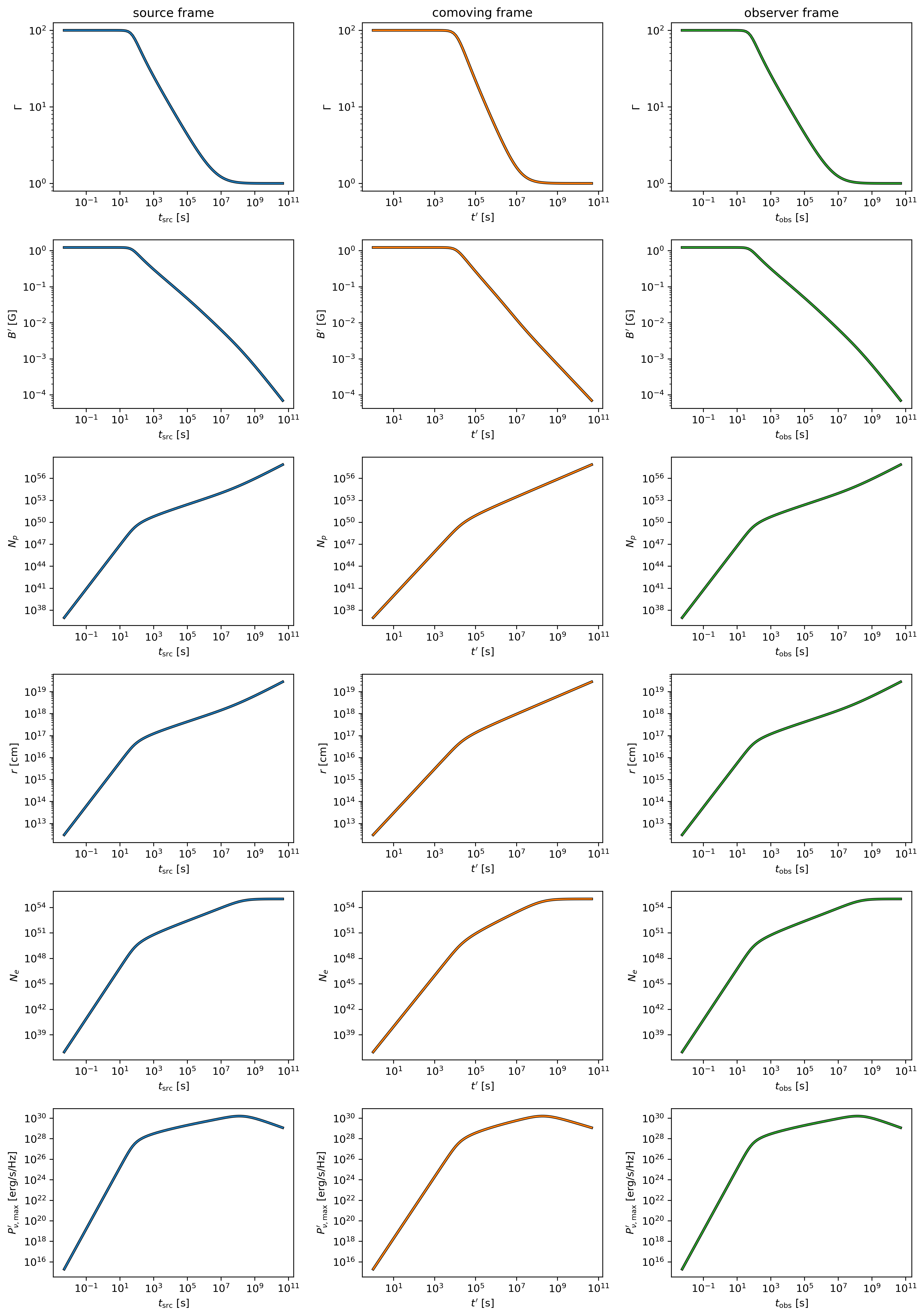
Multi-parameter evolution showing fundamental shock parameters across three reference frames.

Electron Energy Distribution Analysis

This visualization focuses specifically on the characteristic electron energies (self-absorption, injection, and cooling) in both the comoving frame and observer frame, illustrating the relativistic transformation effects:

frames = ['t_src', 't_comv', 't_obs']
xlabels = [r'$t_{\rm src}$ [s]', r'$t^\prime$ [s]', r'$t_{\rm obs}$ [s]']
plt.figure(figsize= (4.2*len(frames), 3.6))

for i, frame in enumerate(frames):
    plt.subplot(1, len(frames), i + 1)
    if frame == 't_src':
        t = getattr(details, frame)
    else:
        t = getattr(details.fwd, frame)
    plt.loglog(t[0, 0, :], details.fwd.gamma_a[0, 0, :],label=r'$\gamma_a^\prime$',c='firebrick')
    plt.loglog(t[0, 0, :], details.fwd.gamma_m[0, 0, :],label=r'$\gamma_m^\prime$',c='yellowgreen')
    plt.loglog(t[0, 0, :], details.fwd.gamma_c[0, 0, :],label=r'$\gamma_c^\prime$',c='royalblue')
    plt.loglog(t[0, 0, :], details.fwd.gamma_a[0, 0, :]*details.fwd.Doppler[0,0,:]/(1+z),label=r'$\gamma_a$',ls='--',c='firebrick')
    plt.loglog(t[0, 0, :], details.fwd.gamma_m[0, 0, :]*details.fwd.Doppler[0,0,:]/(1+z),label=r'$\gamma_m$',ls='--',c='yellowgreen')
    plt.loglog(t[0, 0, :], details.fwd.gamma_c[0, 0, :]*details.fwd.Doppler[0,0,:]/(1+z),label=r'$\gamma_c$',ls='--',c='royalblue')
    plt.xlabel(xlabels[i])
    plt.ylabel(r'$\gamma_e^\prime$')
    plt.legend(ncol=2)
plt.tight_layout()
plt.savefig('electron_quantities.png', dpi=300,bbox_inches='tight')

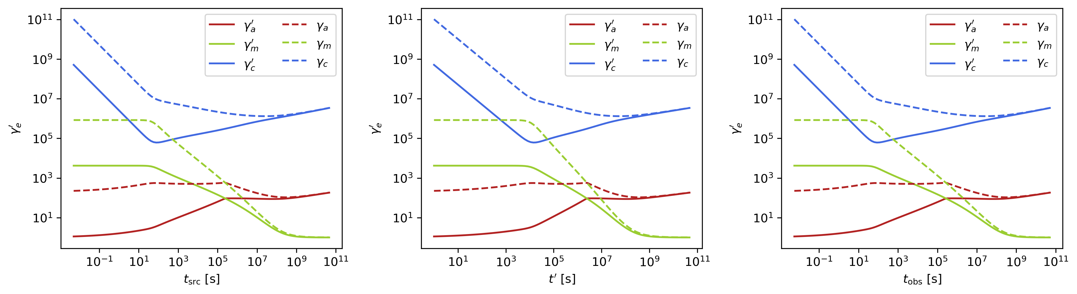
Evolution of characteristic electron energies showing relativistic transformation effects.

Synchrotron Frequency Evolution

This analysis tracks the evolution of characteristic synchrotron frequencies, demonstrating how the spectral break frequencies change over time and how Doppler boosting affects the observed spectrum:

frames = ['t_src', 't_comv', 't_obs']
xlabels = [r'$t_{\rm src}$ [s]', r'$t^\prime$ [s]', r'$t_{\rm obs}$ [s]']
plt.figure(figsize= (4.2*len(frames), 3.6))

for i, frame in enumerate(frames):
    plt.subplot(1, len(frames), i + 1)
    if frame == 't_src':
        t = getattr(details, frame)
    else:
        t = getattr(details.fwd, frame)
    plt.loglog(t[0, 0, :], details.fwd.nu_a[0, 0, :],label=r'$\nu_a^\prime$',c='firebrick')
    plt.loglog(t[0, 0, :], details.fwd.nu_m[0, 0, :],label=r'$\nu_m^\prime$',c='yellowgreen')
    plt.loglog(t[0, 0, :], details.fwd.nu_c[0, 0, :],label=r'$\nu_c^\prime$',c='royalblue')
    plt.loglog(t[0, 0, :], details.fwd.nu_a[0, 0, :]*details.fwd.Doppler[0,0,:]/(1+z),label=r'$\nu_a$',ls='--',c='firebrick')
    plt.loglog(t[0, 0, :], details.fwd.nu_m[0, 0, :]*details.fwd.Doppler[0,0,:]/(1+z),label=r'$\nu_m$',ls='--',c='yellowgreen')
    plt.loglog(t[0, 0, :], details.fwd.nu_c[0, 0, :]*details.fwd.Doppler[0,0,:]/(1+z),label=r'$\nu_c$',ls='--',c='royalblue')
    plt.xlabel(xlabels[i])
    plt.ylabel(r'$\nu$ [Hz]')
    plt.legend(ncol=2)
plt.tight_layout()
plt.savefig('photon_quantities.png', dpi=300,bbox_inches='tight')

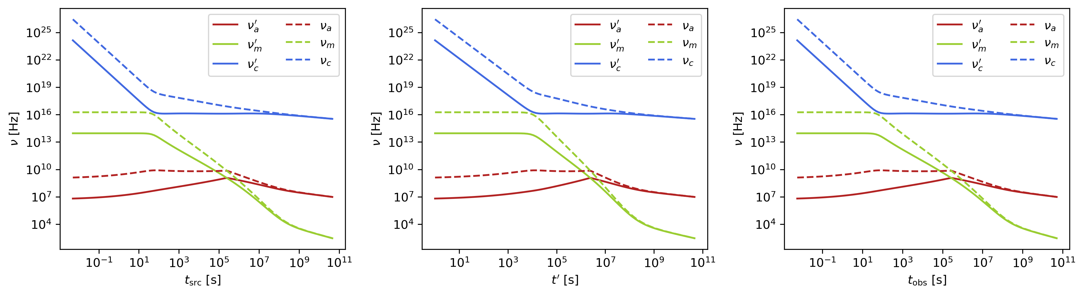
Evolution of characteristic synchrotron frequencies showing spectral break evolution and Doppler effects.

Doppler Factor Spatial Distribution

This polar plot visualizes the spatial distribution of the Doppler factor across the jet structure, showing how relativistic beaming varies with angular position and radial distance:

plt.figure(figsize=(6,6))
ax = plt.subplot(111, polar=True)

theta = details.fwd.theta[0,:,:]
r     = details.fwd.r[0,:,:]
D     = details.fwd.Doppler[0,:,:]

# Polar contour plot
scale = 3.0
c = ax.contourf(theta*scale, r, np.log10(D), levels=30, cmap='viridis')

ax.set_rscale('log')
true_ticks = np.linspace(0, 0.3, 6)
ax.set_xticks(true_ticks * scale)
ax.set_xticklabels([f"{t:.2f}" for t in true_ticks])
ax.set_xlim(0,0.3*scale)
ax.set_ylabel(r'$\theta$ [rad]')
ax.set_xlabel(r'$r$ [cm]')

plt.colorbar(c, ax=ax, label=r'$\log_{10} D$')
plt.tight_layout()
plt.savefig('doppler.png', dpi=300,bbox_inches='tight')

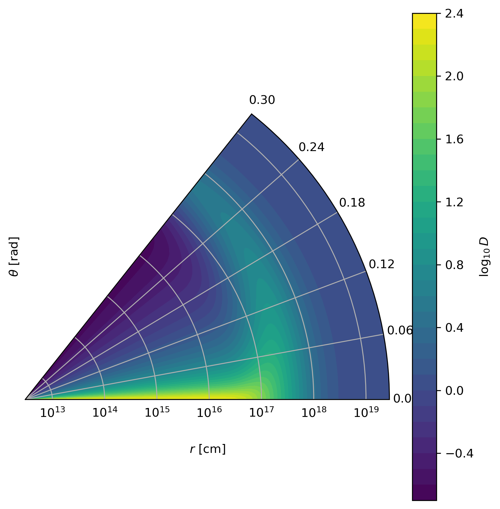
Spatial distribution of Doppler factor showing relativistic beaming effects across the jet structure.

Equal Arrival Time Surface Visualization

This final visualization maps the equal arrival time surfaces in polar coordinates, illustrating how light from different parts of the jet reaches the observer at the same time, which is crucial for understanding light curve morphology:

plt.figure(figsize=(6,6))
ax = plt.subplot(111, polar=True)

theta = details.fwd.theta[0,:,:]
r     = details.fwd.r[0,:,:]
t_obs = details.fwd.t_obs[0,:,:]

scale = 3.0
c = ax.contourf(theta*scale, r, np.log10(t_obs), levels=30, cmap='viridis')

ax.set_rscale('log')
true_ticks = np.linspace(0, 0.3, 6)
ax.set_xticks(true_ticks * scale)
ax.set_xticklabels([f"{t:.2f}" for t in true_ticks])
ax.set_xlim(0,0.3*scale)
ax.set_ylabel(r'$\theta$ [rad]')
ax.set_xlabel(r'$r$ [cm]')

plt.colorbar(c, ax=ax, label=r'$\log_{10} (t_{\rm obs}/s)$')
plt.tight_layout()
plt.savefig('EAT.png', dpi=300,bbox_inches='tight')

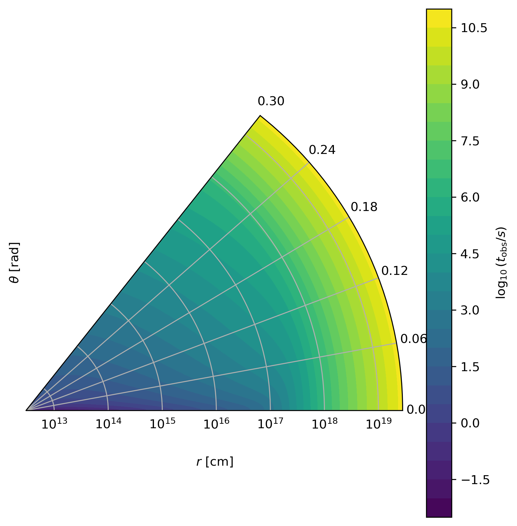
Equal arrival time surfaces showing how light travel time effects determine light curve morphology.

Per-Cell Spectrum Evaluation

In addition to scalar quantities, details() provides callable spectrum accessors that let you evaluate the comoving-frame synchrotron, SSC, and Compton-Y spectra at arbitrary frequencies for each grid cell. To use SSC and Y spectrum, enable SSC in the radiation model:

rad = Radiation(eps_e=1e-1, eps_B=1e-3, p=2.3, ssc=True)
model = Model(jet=jet, medium=medium, observer=obs, fwd_rad=rad, resolutions=(0.15,0.5,10))
details = model.details(t_min=1e0, t_max=1e8)

nu_comv = np.logspace(8, 20, 200)  # comoving frame frequency [Hz]

# Synchrotron spectrum at cell (phi=0, theta=0, t=5)
I_syn = details.fwd.sync_spectrum[0, 0, 5](nu_comv)   # erg/s/Hz/cm²/sr

# SSC spectrum at the same cell (requires ssc=True)
I_ssc = details.fwd.ssc_spectrum[0, 0, 5](nu_comv)    # erg/s/Hz/cm²/sr

# Compton-Y parameter as a function of electron Lorentz factor
gamma = np.logspace(1, 8, 200)
Y = details.fwd.Y_spectrum[0, 0, 5](gamma)            # dimensionless

These callable accessors are also available on details.rvs when a reverse shock is configured. The sync_spectrum and Y_spectrum are always available; ssc_spectrum is None unless ssc=True.

Callable spectrum properties:

• details.fwd.sync_spectrum[i, j, k](nu_comv): Comoving synchrotron specific intensity at given frequencies. Input: comoving frequency in Hz. Output: \(I_\nu\) in erg/s/Hz/cm²/sr.

• details.fwd.ssc_spectrum[i, j, k](nu_comv): Comoving SSC specific intensity. Same units as synchrotron. Only available when ssc=True.

• details.fwd.Y_spectrum[i, j, k](gamma): Compton-Y parameter as a function of electron Lorentz factor. Input: dimensionless \(\gamma\). Output: dimensionless \(Y(\gamma)\).

Model Configuration Introspection

VegasAfterglow provides introspection methods to examine jet and medium properties at specific coordinates. These methods are useful for understanding model configuration, validating parameters, and creating diagnostic plots.

Jet Property Introspection

You can examine the angular dependence of jet properties using the jet_E_iso and jet_Gamma0 methods:

import numpy as np
import matplotlib.pyplot as plt
from VegasAfterglow import PowerLawJet, ISM, Observer, Radiation, Model

# Create a power-law jet for demonstration
jet = PowerLawJet(theta_c=0.1, E_iso=1e52, Gamma0=300, k_e=2.0, k_g=1.5)
medium = ISM(n_ism=1)
obs = Observer(lumi_dist=1e26, z=0.1, theta_obs=0)
rad = Radiation(eps_e=1e-1, eps_B=1e-3, p=2.3)
model = Model(jet=jet, medium=medium, observer=obs, fwd_rad=rad)

# Define angular coordinates
phi = 0.0  # Azimuthal angle (for axisymmetric jets, phi doesn't matter)
theta = np.linspace(0, 0.5, 100)  # Polar angles from 0 to 0.5 radians

# Get jet properties
E_iso_profile = model.jet_E_iso(phi, theta)  # Isotropic energy [erg]
Gamma0_profile = model.jet_Gamma0(phi, theta)  # Initial Lorentz factor

# Create visualization
fig, (ax1, ax2) = plt.subplots(1, 2, figsize=(10, 4))

# Plot energy profile
ax1.semilogy(np.degrees(theta), E_iso_profile)
ax1.set_xlabel('Polar Angle [degrees]')
ax1.set_ylabel(r'$E_{\rm iso}$ [erg]')
ax1.set_title('Jet Energy Profile')
ax1.grid(True, alpha=0.3)

# Plot Lorentz factor profile
ax2.semilogy(np.degrees(theta), Gamma0_profile)
ax2.set_xlabel('Polar Angle [degrees]')
ax2.set_ylabel(r'$\Gamma_0$')
ax2.set_title('Jet Lorentz Factor Profile')
ax2.grid(True, alpha=0.3)

plt.tight_layout()
plt.show()

Medium Density Introspection

You can examine the radial dependence of medium density using the medium method:

from VegasAfterglow import Wind

# Create a wind medium for demonstration
wind = Wind(A_star=1.0, n_ism=0.1, n0=1e3, k=2)
# Note: This creates a stratified wind: inner constant density n0,
# middle r^-2 profile, outer constant density n_ism

# Create model with wind medium
model = Model(jet=jet, medium=wind, observer=obs, fwd_rad=rad)

# Define radial coordinates
phi = 0.0
theta = 0.1  # 0.1 radians off-axis
r = np.logspace(15, 20, 100)  # Radii from 10^15 to 10^20 cm

# Get medium density profile
rho_profile = model.medium(phi, theta, r)  # Density [g/cm³]

# Convert to number density (assuming pure hydrogen)
n_profile = rho_profile / (1.67e-24)  # [cm^-3]

# Create visualization
plt.figure(figsize=(8, 6))
plt.loglog(r, n_profile)
plt.xlabel(r'Radius [cm]')
plt.ylabel(r'Number Density [cm$^{-3}$]')
plt.title('Medium Density Profile')
plt.grid(True, alpha=0.3)

# Add annotations for different regions
plt.axhline(1e3, color='red', linestyle='--', alpha=0.7, label='Inner constant density')
plt.axhline(0.1, color='blue', linestyle='--', alpha=0.7, label='Outer ISM density')
plt.legend()
plt.show()

Two-Component Jet Analysis

For complex jet structures like two-component jets, introspection is particularly useful:

from VegasAfterglow import TwoComponentJet

# Create a two-component jet
jet = TwoComponentJet(
    theta_c=0.05,    # Narrow component
    E_iso=1e53,
    Gamma0=300,
    theta_w=0.15,    # Wide component
    E_iso_w=1e52,
    Gamma0_w=100
)

model = Model(jet=jet, medium=medium, observer=obs, fwd_rad=rad)

# Examine the jet structure
theta = np.linspace(0, 0.3, 200)
E_iso_profile = model.jet_E_iso(0, theta)
Gamma0_profile = model.jet_Gamma0(0, theta)

# Create detailed visualization
fig, (ax1, ax2) = plt.subplots(2, 1, figsize=(8, 8))

# Energy profile
ax1.semilogy(np.degrees(theta), E_iso_profile)
ax1.axvline(np.degrees(0.05), color='red', linestyle='--', alpha=0.7, label='Core boundary')
ax1.axvline(np.degrees(0.15), color='blue', linestyle='--', alpha=0.7, label='Wide component boundary')
ax1.set_ylabel(r'$E_{\rm iso}$ [erg]')
ax1.set_title('Two-Component Jet: Energy Profile')
ax1.legend()
ax1.grid(True, alpha=0.3)

# Lorentz factor profile
ax2.semilogy(np.degrees(theta), Gamma0_profile)
ax2.axvline(np.degrees(0.05), color='red', linestyle='--', alpha=0.7, label='Core boundary')
ax2.axvline(np.degrees(0.15), color='blue', linestyle='--', alpha=0.7, label='Wide component boundary')
ax2.set_xlabel('Polar Angle [degrees]')
ax2.set_ylabel(r'$\Gamma_0$')
ax2.set_title('Two-Component Jet: Lorentz Factor Profile')
ax2.legend()
ax2.grid(True, alpha=0.3)

plt.tight_layout()
plt.show()

These introspection methods are essential for:

• Model validation: Ensuring jet and medium configurations match your intentions

• Parameter studies: Understanding how changes in parameters affect the structure

• Publication plots: Creating clean visualizations of model configurations

• Debugging: Identifying issues with complex multi-component setups

• Physical understanding: Gaining insight into the initial conditions of your simulations